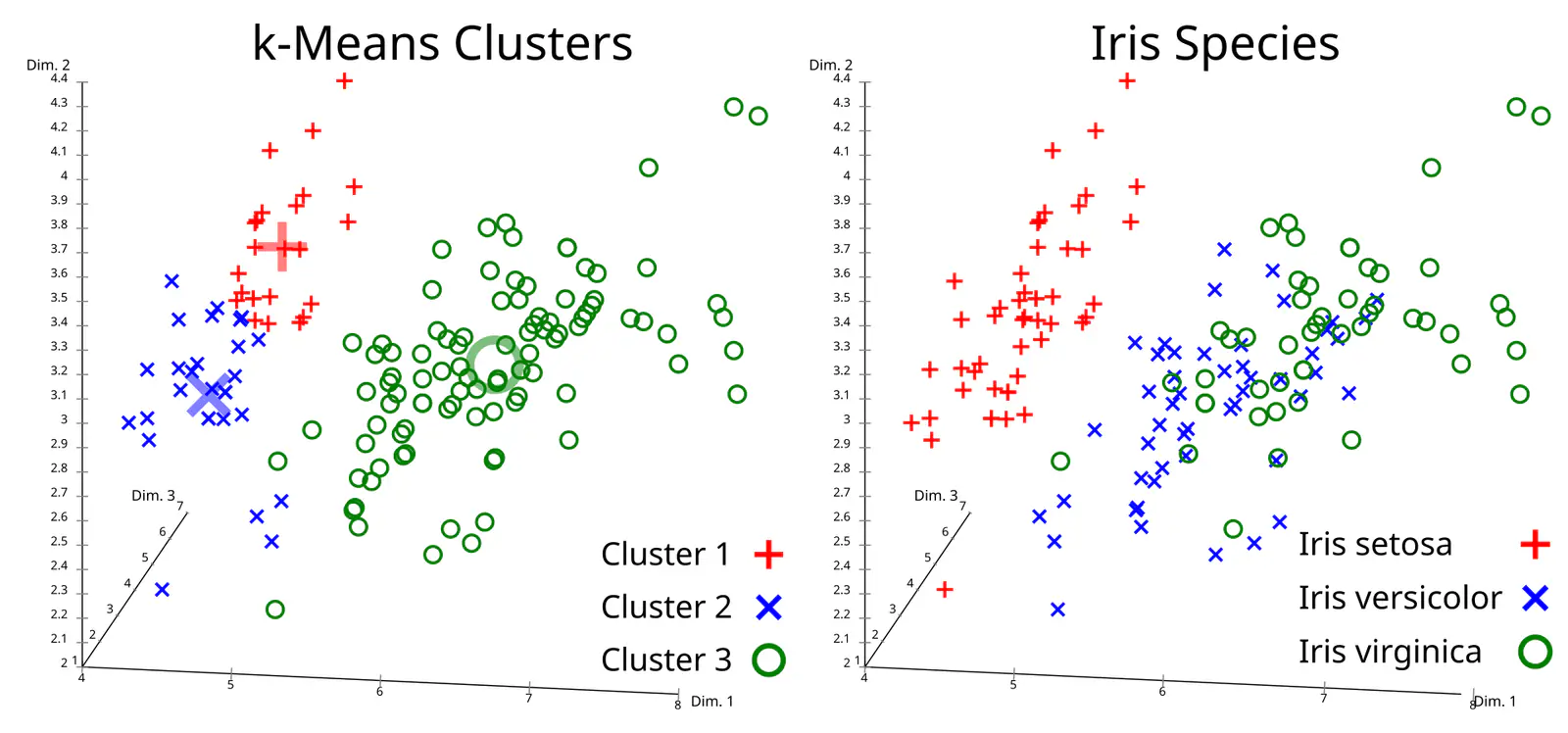
K-means clustering is an algorithm that splits a set of data points into a chosen number k of groups, by repeatedly assigning each point to its nearest group center and then moving each center to the average of its points. The standard version was described by Stuart Lloyd at Bell Labs in 1957 and published in IEEE Transactions on Information Theory in 1982, and in 2007 David Arthur and Sergei Vassilvitskii added the k-means++ seeding step that most libraries now use by default. It remains the default first clustering method because it is simple, fast and easy to explain.
What k-means is trying to minimize
K-means is a form of unsupervised learning: it receives points without labels and has to find structure by itself. Given the data and an integer k, it returns k centers, called centroids, and a cluster label for every point.
The quantity it tries to make small is the sum of squared distances from each point to its closest centroid. scikit-learn calls this “inertia” or the within-cluster sum of squares; the k-means++ paper calls it the potential, φ. It has no fixed scale, so it only compares runs on the same data. Finding the true minimum is NP-hard even for two clusters, as Arthur and Vassilvitskii note, so practice relies on fast local search.
How Lloyd’s algorithm works
The local search people simply call “k-means” is Lloyd’s algorithm. According to Wikipedia’s history of the method, Lloyd developed it in 1957 for pulse-code modulation, the task of representing an analog signal with a small set of discrete levels; Edward Forgy published essentially the same method in 1965, and James MacQueen coined the term “k-means” in 1967. The loop has three parts:
- Initialize. Pick k starting centroids. The most basic method takes k random points from the data.
- Assign. Give every point to its nearest centroid. Geometrically, this cuts space into one region per centroid, a Voronoi diagram.
- Update. Move each centroid to the mean of the points assigned to it.
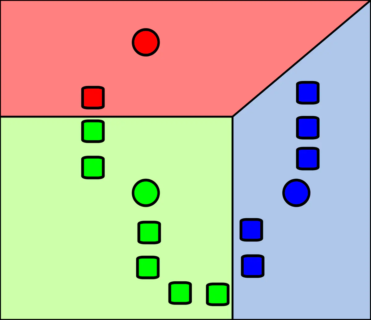
Steps 2 and 3 repeat until the centroids barely move. Each step can only lower the squared error, so no clustering repeats, and because there are finitely many ways to split the points, the loop always stops. The catch is that it stops at a local minimum, which may be far from the best possible clustering, and which minimum it lands in depends on where it started.
A worked example: six numbers, two clusters
Take six values on a line, 1, 2, 4, 9, 10 and 12, with k = 2. The natural split is {1, 2, 4} and {9, 10, 12}. Suppose the algorithm starts badly, with both centroids at the low end: 1 and 2.
Iteration 1, assign. Point 1 goes to centroid 1. Every other point (2, 4, 9, 10, 12) is closer to centroid 2. The squared error at this moment is 0 + 0 + 4 + 49 + 64 + 100 = 217.
Iteration 1, update. Centroid 1 stays at 1. Centroid 2 moves to the mean of its five points: (2 + 4 + 9 + 10 + 12) / 5 = 7.4. The squared error falls to 71.2.
Iteration 2, assign. The boundary between the centroids is now halfway between 1 and 7.4, at 4.2. So 1, 2 and 4 join the first cluster, and 9, 10 and 12 join the second.
Iteration 2, update. The new centroids are 7 / 3 ≈ 2.33 and 31 / 3 ≈ 10.33. Each cluster contributes about 4.67 to the squared error, for a total of about 9.33.
Iteration 3. The new boundary sits at about 6.33, and no point changes sides, so the algorithm has converged. The error fell from 217 to 71.2 to 9.33, exactly the monotone behavior the theory promises.
Here the bad start still found the natural split, but on messier data a poor start can leave two centroids sharing one real group while another group gets none. That is the problem k-means++ addresses.
How k-means++ picks better starting points
Arthur and Vassilvitskii’s fix changes only the initialization. The first centroid is a random data point. Each later centroid is drawn at random, but with probability proportional to D(x)², the squared distance from a point to the nearest centroid already chosen. Points far from existing centers become much more likely picks, so the seeds spread out.

In our example, if the first seed is 1, the squared distances of the six points to it are 0, 1, 9, 64, 81 and 121, adding up to 276. The three points in the upper group account for 266 of that, so the second seed lands in the right group about 96% of the time, instead of 50% with uniform random picks.
The paper proves the expected error is then at most 8(ln k + 2) times the optimum, a guarantee random seeding lacks, and reports that it also made k-means faster and more accurate in experiments. scikit-learn uses k-means++ by default; its documentation says it implements a “greedy” variant that tries several candidates at each sampling step and keeps the best one.
Where k-means breaks down
Its objective bakes in assumptions that the scikit-learn user guide spells out:
- It expects round, similar-sized clusters. Inertia assumes clusters are convex and isotropic, so k-means handles elongated or irregularly shaped groups poorly.
- Distances get inflated in high dimensions. The guide recommends reducing dimensions first, for example with principal component analysis, which can also speed up computation.
- You must choose k. It returns as many clusters as you ask for. Silhouette analysis is a common way to compare choices of k, while the popular “elbow” plot is, as Wikipedia notes, loosely defined and often unreliable.
- Results depend on the start. Libraries therefore run it several times. In scikit-learn the
n_initsetting defaults to “auto”, which means one run with k-means++ seeding and ten runs with random seeding, keeping the run with the lowest inertia.
Where k-means fits in today’s AI stack
Lloyd’s original use, compressing a signal to a few representative values, survives in tasks such as reducing an image to a small color palette. In AI systems, clustering often works behind the scenes: inverted-file (IVF) vector indexes group embeddings into clusters so a query only scans the most promising ones, as our guide to vector databases explains. K-means is also a quick first look at unlabeled business data, such as customer segments. For labeled tabular prediction, by contrast, the tools of choice are usually tree ensembles, as we explained in gradient boosting vs deep learning on tabular data.
What to watch next
- Whether your library’s defaults change: scikit-learn switched
n_initto “auto” in version 1.4, which changes run-to-run behavior. - Use of k-means inside approximate nearest-neighbor indexes as embedding collections grow.
- Alternatives like DBSCAN or HDBSCAN when clusters are irregular or noise is common.
Key takeaways
- K-means splits data into k groups by alternating “assign to nearest centroid” and “move centroid to the mean”.
- Each step lowers the squared error, so it always converges, but only to a local minimum.
- K-means++ seeds centroids with D² weighting and comes with a provable O(log k) bound on expected error.
- It works best on compact, round clusters; elongated shapes, high dimensions and the choice of k are its weak points.
- The algorithm dates to Lloyd’s 1957 Bell Labs work and remains a building block in modern AI tooling.
Frequently asked questions
What is k-means clustering used for?
It groups unlabeled data into a chosen number of clusters, for tasks such as customer segmentation, reducing image color palettes and exploring a new dataset.
Does k-means always find the best clusters?
No. It always converges, but to a local minimum that depends on the starting centroids. Running it several times and using k-means++ seeding reduces the risk of a poor result.
How do I choose k in k-means?
There is no single correct method. Silhouette analysis compares how well points fit their own cluster versus neighboring ones across several values of k, and domain knowledge matters just as much.